Bodge tutorial

Abstract

Bodge is a Python package for constructing large real-space tight-binding models. Although quite general tight-binding models can be constructed, we focus on the Bogoliubov-DeGennes (“BoDGe”) Hamiltonian, which is most commonly used to model superconductivity in clean materials and heterostructures. So if you want a lattice model for superconducting nanostructures, and want something that is efficient yet easy to use, then you’ve come to the right place.

Installation

Bodge has been uploaded to the Python Package Index (PyPI). This means that if you have a recent version of Python and Pip installed on your system, installing this package should be as simple as:

pip install bodge

For more installation alternatives, please see the README on GitHub.

Getting started

I believe the easiest way to get started is “learning by doing”, so in this section we jump straight into some examples of how one can use Bodge in practice. This introduction assumes that you are somewhat familiar with tight-binding models in condensed matter physics.

For a better understanding of the mathematics behind these examples, as well as how Bodge handles them internally, please see the more detailed explanations under Mathematical details and Numerical details below. For more advanced usage, I would recommend looking through the source code itself, which is well-documented in the form of docstrings and comments. Some real-world use cases of Bodge live on the development branch, but keep in mind that those functions have not received the same level of polish and testing as the main branch and therefore may contain bugs.

Please note that to follow the examples below, you need to install Matplotlib:

pip install matplotlib

Depending on how you are running the code (e.g. in a Jupyter notebook or in a terminal), you might need to run plt.show() after each example to actually see the generated plots. (Alternatively, plt.savefig('filename.png') to save the plots to file instead.)

Normal metal

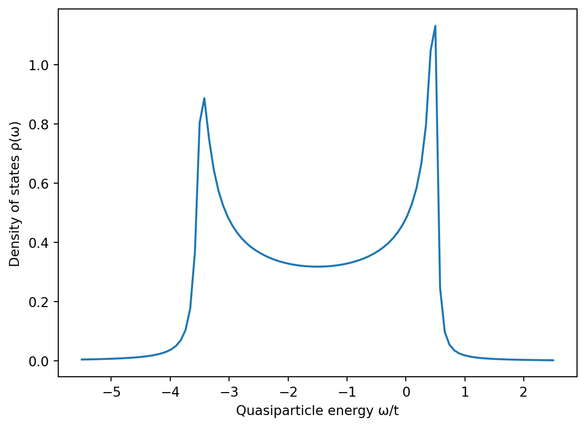
The simplest electronic tight-binding model is arguably a one-dimensional normal-metal wire. As an introductory example, let’s therefore try to calculate the local density of states (LDOS) in the middle of such a wire.

A wire can be considered an \(L_x \times L_y \times L_z\) cubic lattice in the limit that \(L_x \gg L_y = L_z\). The tight-binding model for normal metals contains only a chemical potential \(\mu\) and a hopping amplitude \(t\), and is often written as: \[\mathcal{H} = -\mu \sum_{i\sigma} c^\dagger_{i\sigma} c_{i\sigma} -t \sum_{\langle ij \rangle \sigma} c^\dagger_{i\sigma} c_{j\sigma}.\] Bodge however requires that it be written in the form: \[\mathcal{H} = \sum_{i\sigma\sigma'} c^\dagger_{i\sigma} (H_{ii})_{\sigma\sigma'} c_{i\sigma'} + \sum_{\langle ij \rangle \sigma\sigma'} c^\dagger_{i\sigma} (H_{ij})_{\sigma\sigma'} c_{j\sigma'},\] where \(H_{ii}\) and \(H_{ij}\) are \(2\times2\) matrices that represents spin dependence. From this, we basically see that the system above can be summarized as: \[H_{ij} = \begin{cases} -\mu\sigma_0 & \text{if $i = j$,} \\ -t\sigma_0 & \text{otherwise.} \end{cases}\] This is precisely what we need to tell Bodge to create the desired Hamiltonian. The following code performs the calculations we want:

# Standard imports in every numerical Python code
import numpy as np
import matplotlib.pyplot as plt

# Bodge is designed to be imported in this way, but you can
# of course `import bodge as bdg` if you really want to
from bodge import *

# Define the tight-binding model parameters
Lx = 512
Ly = 1
Lz = 1

t = 1
μ = 1.5 * t

# Construct the Hamiltonian
lattice = CubicLattice((Lx, Ly, Lz))
system = Hamiltonian(lattice)

with system as (H, _):
    for i in lattice.sites():
        H[i, i] = -μ * σ0
    for i, j in lattice.bonds():
        H[i, j] = -t * σ0

# If you need the Hamiltonian matrix itself, you could use:
# H = system.matrix()  # NumPy dense array
# H = system.matrix(format="csr")  # SciPy sparse matrix

# Calculate the central density of states
i = (Lx//2, Ly//2, Lz//2)
ω = np.linspace(-μ-4*t, -μ+4*t, 101)
ρ = system.ldos(i, ω)

# Plot the density of states at the system center
plt.figure()
plt.xlabel("Quasiparticle energy ω/t")
plt.ylabel("Density of states ρ(ω)")
plt.plot(ω, ρ)

Some things I want to elaborate on in this example:

• Bodge implements a “context manager” for filling out terms H[i, j] in the Hamiltonian. So every time you want to update the Hamiltonian, you write a with system as ...: block, after which you can pretend that H[i, j] simply indexes a large Hamiltonian matrix. Once you exit the with block, Bodge takes care of the gory details: Transferring the terms in the Hamiltonian to the underlying sparse matrix, ensuring that Hermitian and particle-hole symmetries are satisfied, and complaining loudly if the Hamiltonian is non-Hermitian. As mentioned in the comments, you can at this point use the system.matrix() method to obtain the constructed Hamiltonian matrix if you need it.
• Note that everything you insert using H[i, j] = ... must be a \(2\times2\) complex matrix, which is most easily done by multiplying coefficients with one of the Pauli matrices σ0, σ1, σ2, σ3, or their complex equivalents jσ0 = 1j * σ0 etc. These symbols are automatically imported when you do from bodge import *. I like to code using Greek letters to use the same notation in papers and code – Python supports Unicode variable names, and typing them is usually straight-forward.¹ But if you don’t want Unicode symbols, that is completely fine as well: Bodge doesn’t require Unicode anywhere. Every object exported by the library has an ASCII version, so you can e.g. type sigma0 and jsigma2 instead of σ0 and jσ2 if you prefer that.
• When filling out the matrix, we can use lattice.sites() and lattice.bonds() to iterate over the whole lattice. In this case, we have kept it simple, and only have one type of on-site term and one type of hopping term, but Bodge itself is very flexible. You can e.g. use lattice.bonds(axis=0) to iterate over only bonds that point along the 0th axis (x axis), which is useful if you need different hopping terms in different directions. Moreover, each coordinate \(i\) above is simply a tuple \((x_i, y_i, z_i)\) where \(0 \leq x_i < L_x\) and so on. Thus, you can use e.g. if i[0] < Lx/2: to implement a sharp interface between different materials, or a function call like np.sin(np.pi*i[0]/Lx) to implement a field that varies smoothly throughout the lattice.
• The system.ldos method implements an efficient sparse matrix algorithm to obtain the local density of states at a single site \(i\). The algorithm implemented is explained in detail in Appendix A of this paper, and is essentially a simplified version of the algorithm from this paper. You could alternatively diagonalize the Hamiltonian using E, X = system.diagonalize(), and then use the eigenvalues E[n] and corresponding eigenvectors X[n,:,:] to obtain the density of states as described in e.g. Zhu’s textbook. However, this approach uses dense matrices (NumPy arrays), and is therefore significantly slower for large systems. I’d therefore recommend researching whether you can use a sparse matrix algorithm before you diagonalize large matrices.

Conventional superconductor

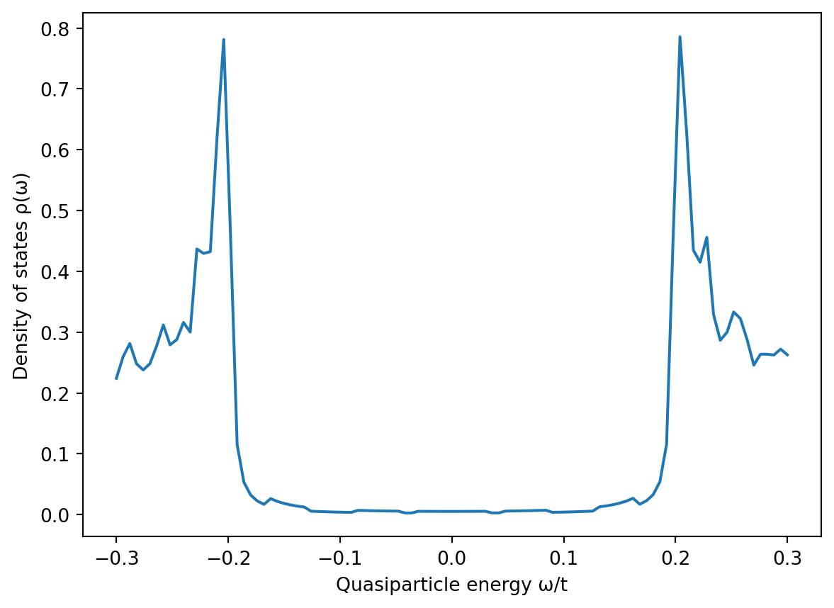
Let’s now consider a two-dimensional conventional (BCS) superconductor, which has an \(s\)-wave singlet order parameter \(Δ_s\). In this case, we want to consider a medium-large \(101\times101\) lattice, but are only interested in the density of states in a narrow energy range around the “superconducting gap” at the Fermi level – since this is the part of the energy spectrum that is relevant for most transport phenomena.

Conventional superconductors can be described by a Hamiltonian operator \(\mathcal{H} = \mathcal{H}_N + \mathcal{H}_S\) that contain both the normal-metal contributions \(\mathcal{H}_N\) described under normal metal and an additional pairing term \[\mathcal{H}_S = -\sum_{i\sigma\sigma'} c^\dagger_{i\sigma} (\Delta_s i\sigma_2)_{\sigma\sigma'} c^\dagger_{i\sigma'} + \text{h.c.,}\] where \(\Delta_s\) is a complex number that can in general be a function of position. The matrix \(i\sigma_2\) simply produces a spin structure of the form \(\uparrow\downarrow - \downarrow\uparrow\), which is appropriate for a spin-singlet state.

To model this using Bodge, we simply use a with system as (H, Δ) block to access the Hamiltonian object, and set the on-site terms Δ[i, i] to the contents \(\Delta_s i\sigma_2\) of the parentheses above:

import numpy as np
import matplotlib.pyplot as plt

from bodge import *

# Model parameters
Lx = 201
Ly = 201

t = 1
μ = -3 * t
Δs = 0.2 * t

# Construct the Hamiltonian
lattice = CubicLattice((Lx, Ly, 1))
system = Hamiltonian(lattice)

with system as (H, Δ):
    for i in lattice.sites():
        H[i, i] = -μ * σ0
        Δ[i, i] = -Δs * jσ2
    for i, j in lattice.bonds():
        H[i, j] = -t * σ0

# Calculate the density of states
i = (Lx//2, Ly//2, 0)
ω = np.linspace(-1.5 * Δs, 1.5 * Δs, 101)
ρ = system.ldos(i, ω)

# Plot the results
plt.figure()
plt.xlabel("Quasiparticle energy ω/t")
plt.ylabel("Density of states ρ(ω)")
plt.plot(ω, ρ)

The rest of the code is the same as for the normal metal. We correctly get a “superconducting gap” of width \(2Δ_s\) at the Fermi level \(\omega=0\).

It is also quite straight-forward if you want to consider a current-carrying superconductor: you just need to introduce a complex phase winding into the superconducting gap. For instance, to get one full phase winding across the system along the \(x\) direction, we can let \(\Delta_s \to \Delta_s e^{2 \pi i x/L_x}\). To ensure that charge current is conserved at the system’s edges, you may however want to turn on periodic boundary conditions as well. Bodge can facilitate this using another iterator lattice.edges(), which returns pairs of lattice sites (i, j) on opposite ends of the lattice so that we can add hopping terms that “wrap around” the lattice. This is usually a decent model for the behavior of a large bulk superconductor with an applied electric current:

with system as (H, Δ):
    for i in lattice.sites():
        Δi = Δs * np.exp(2*π*1j*i[0]/Lx)
        H[i, i] = -μ * σ0
        Δ[i, i] = -Δi * jσ2
    for i, j in lattice.bonds():
        H[i, j] = -t * σ0
    for i, j in lattice.edges():
        H[i, j] = -t * σ0

Unconventional superconductors

In unconventional superconductors, the electrons that form a Cooper pair reside on different lattice sites. Moreover, they often have a complex dependence on directionality, such that pairing terms along different cardinal axes on the lattice have different complex phases. Generally, this kind of pairing term contributes as follows to the Hamiltonian: \[\mathcal{H}_S = -\sum_{\langle ij \rangle \sigma\sigma'} c^\dagger_{i\sigma} (\Delta_{ij})_{\sigma\sigma'} c^\dagger_{j\sigma'} + \text{h.c.,}\] where we have to specify some pairing function \(\Delta_{ij}\).

One example of such a state is a “\(d\)-wave singlet superconductor”, which describes e.g. high-temperature cuprates. This can be modeled as: \[\Delta_{ij} = \begin{cases} -\Delta_d i\sigma_2 & \text{if $i, j$ are neighbors along the $x$ axis,}\\ +\Delta_d i\sigma_2 & \text{if $i, j$ are neighbors along the $y$ axis.}\end{cases}\] Implementing this kind of system in Bodge is straight-forward:

Δd = 0.1 * t
with system as (H, Δ):
    for i, j in lattice.bonds():
        H[i, j] = -t * σ0
    for i, j in lattice.bonds(axis=0):
        Δ[i, j] = -Δd * jσ2
    for i, j in lattice.bonds(axis=1):
        Δ[i, j] = +Δd * jσ2

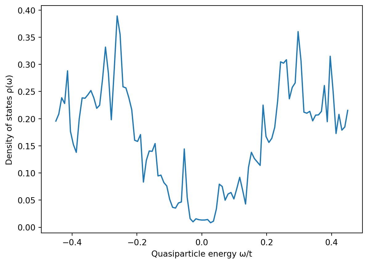
For “\(p\)-wave triplet superconductors”, the pairing \(\Delta_{ij}\) can become very complicated due to the many different degrees of freedom involved. In the literature, this is often described in terms of a \(d\)-vector: \(\Delta_{ij} = [\mathbf{d}(\mathbf{p})\cdot\boldsymbol{\sigma}]i\sigma_2\) where \(\mathbf{d}(\mathbf{p})\) is a linear-in-momentum function that describes the spin dependence. Bodge can take in a \(d\)-vector expression like e.g. \(\mathbf{d}(\mathbf{p}) = \mathbf{e}_z p_x\) and construct the correct matrix expression for \(\Delta_{ij}\) for you. Here is an example:

import numpy as np
import matplotlib.pyplot as plt

from bodge import *

# Model parameters
Lx = 101
Ly = 101

t = 1
μ = -3 * t
Δp = 0.3 * t

# Construct the Hamiltonian
lattice = CubicLattice((Lx, Ly, 1))
system = Hamiltonian(lattice)

σp = pwave("e_z * p_x")

with system as (H, Δ):
    for i in lattice.sites():
        H[i, i] = -μ * σ0
    for i, j in lattice.bonds():
        H[i, j] = -t * σ0
        Δ[i, j] = -Δp * σp(i, j)

# Calculate the density of states
i = (Lx//2, Ly//2, 0)
ω = np.linspace(-1.5 * Δp, 1.5 * Δp, 101)
ρ = system.ldos(i, ω)

# Plot the results
plt.figure()
plt.xlabel("Quasiparticle energy ω/t")
plt.ylabel("Density of states ρ(ω)")
plt.plot(ω, ρ)

More complex \(d\)-vector expressions are also possible; for instance, you can use pwave("(e_x + je_y) * (p_x + jp_y) / 2") to get a non-unitary chiral \(p\)-wave state. The main “rule” is that you need to write the \(d\)-vector in a form where all the unit vectors \(\{ \mathbf{e}_x, \mathbf{e}_y, \mathbf{e}_z \}\) are written to the left of the momentum variables \(\{ p_x, p_y, p_z \}\). The algorithm used in pwave is described in Sec. II-B of this paper.

In addition to the pwave function, Bodge provides a dwave function for modeling \(d_{x^2-y^2}\) superconductors and an swave function for consistency. However, for singlet superconductors, you may find it easier to encode the tight-binding model “manually” as shown above.

Magnetic materials

Let us now consider a superconductor exposed to a strong magnetic field, where the Zeeman effect can result in a spin splitting. Alternatively, the same physics would arise in e.g. superconductor/ferromagnet bilayers, and Bodge can model these as well (you just need some simple if tests to determine which fields apply to which lattice sites).

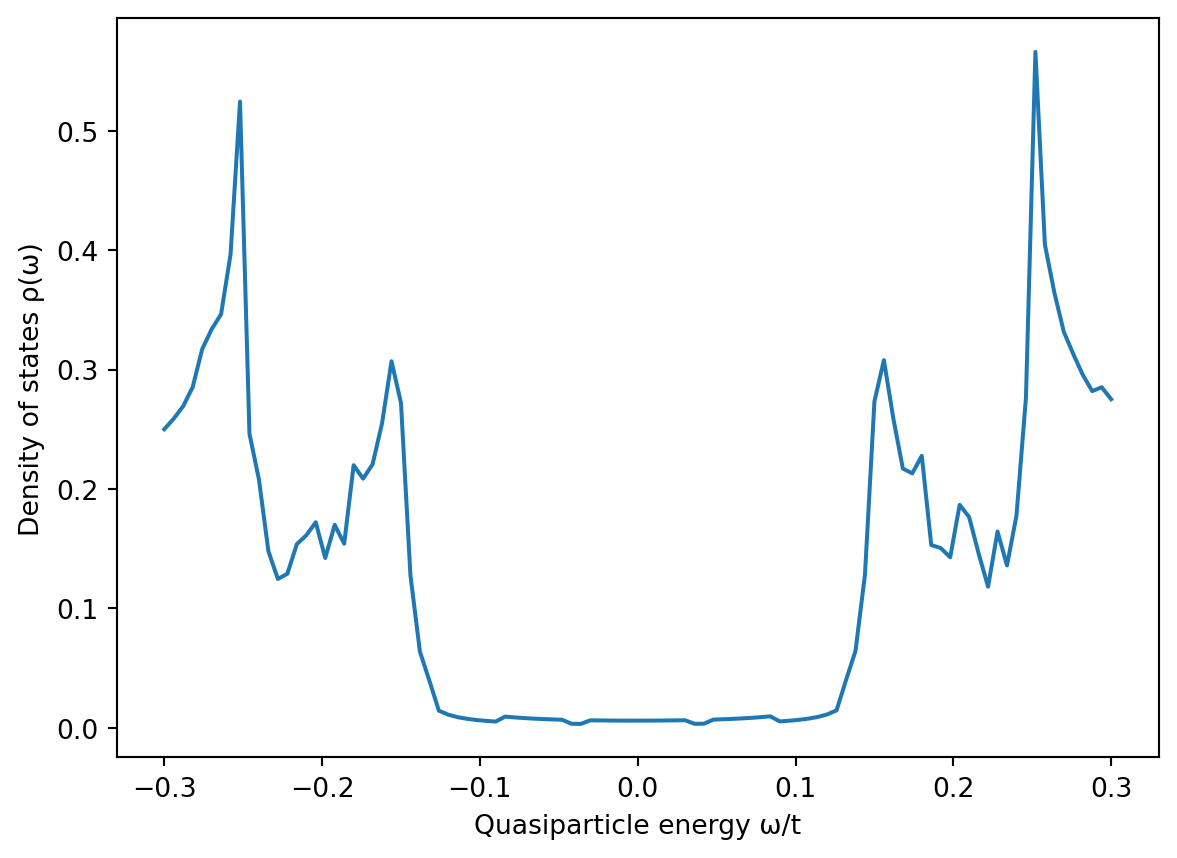
Magnetism can be modeled by introducing a spin-dependent term \(-\mathbf{M} \cdot \boldsymbol{\sigma}\) into the on-site Hamiltonian \(H_{ii}\). In the simple case \(\mathbf{M} = M_z \mathbf{e}_z\) of a homogeneous magnetic field, we are simply left with a term \(-M_z \sigma_3\) in the Hamiltonian. Modifying the code for the conventional superconductor, we get:

import numpy as np
import matplotlib.pyplot as plt

from bodge import *

# Model parameters
Lx = 201
Ly = 201

t = 1
μ = -3.0 * t
Δs = 0.20 * t
Mz = 0.25 * Δs

# Construct the Hamiltonian
lattice = CubicLattice((Lx, Ly, 1))
system = Hamiltonian(lattice)

with system as (H, Δ):
    for i in lattice.sites():
        H[i, i] = -μ * σ0 - Mz * σ3
        Δ[i, i] = -Δs * jσ2
    for i, j in lattice.bonds():
        H[i, j] = -t * σ0

# Calculate the density of states
i = (Lx//2, Ly//2, 0)
ω = np.linspace(-1.5 * Δs, 1.5 * Δs, 101)
ρ = system.ldos(i, ω)

# Plot the results
plt.figure()
plt.xlabel("Quasiparticle energy ω/t")
plt.ylabel("Density of states ρ(ω)")
plt.plot(ω, ρ)

We see that the presence of magnetism causes the well-known “spin splitting” of the density of states, where the sharp peaks at \(\omega = \pm\Delta_s\) are split in two. The strength of this splitting is given by \(M_z\).

Other forms of spin-dependence are also easily implemented in Bodge:

• Ferromagnetic domain walls can be implemented by setting H[i, i] = -Mx(i) * σ1 - My(i) * σ2 - Mz(i) * σ3 for arbitrary functions \(\{M_x(i), M_y(i), M_z(i)\}\) that depend on the lattice sites \(i = (x_i, y_i, z_i)\).
• Antiferromagnetism can be modeled by letting the spin alternate from site to site. For instance, H[i, i] = -Mz * σ3 * (-1)**sum(i) would create a “checkerboard-patterned” antiferromagnet.
• Altermagnetism and spin-orbit coupling can be modeled by having spin-dependent hopping terms instead of spin-dependent on-site terms. For instance, you can let H[i, j] = -t * σ0 -m * σ3.

Mathematical details

In condensed matter physics, one usually writes the Hamiltonian operator \(\mathcal{H}\) of some physical system in the language of quantum field theory. To describe electrons living in a crystal lattice (e.g. a metal), the basic building blocks we need are an operator \(c_{i\sigma}^\dagger\) that “puts” an electron with spin \(\sigma \in \{\uparrow, \downarrow\}\) at a lattice site described by some index \(i\), and another operator \(c_{i\sigma}\) that “removes” a corresponding electron from that site. One can describe many physical phenomena in this way. For instance, a product \(c^\dagger_{1,\uparrow} c_{2,\downarrow}^{\phantom{\dagger}}\) of two such operators would remove a spin-down electron from site \(2\) and place a spin-up electron at site \(1\): this models an electron that jumps between two lattice sites while flipping its spin. After summing many terms like this, the Hamiltonian operator \(\mathcal{H}\) will contain a complete description of the permitted processes in our model – which can then be used to determine the system’s ground state, order parameters, electric currents, and other properties of interest.

We here focus on systems that can harbor superconductivity, which is often modeled using variants of the “Bogoliubov-deGennes Hamiltonian”. In a very general form, such a Hamiltonian operator can be written: \[\mathcal{H} = E_0 + \frac{1}{2} \sum_{ij} \hat{c}^\dagger_i \hat{H}_{ij} \hat{c}_j,\] where \(\hat{c}_i = (c_{i\uparrow}, c_{i\downarrow}, c_{i\uparrow}^\dagger, c_{i\downarrow}^\dagger)\) is a vector of all spin-dependent electron operators on lattice site \(i\). \(E_0\) is a constant that can often be neglected, but can be important if you need to self-consistently determine any order parameters. The \(4\times4\) matrices \(\hat{H}_{ij}\) can be further decomposed into \(2\times2\) blocks \(H_{ij}\) and \(\Delta_{ij}\): \[\hat{H}_{ij} = \begin{pmatrix} H_{ij} & \Delta_{ij} \\ \Delta^\dagger_{ij} & -H^*_{ij} \end{pmatrix}.\] Physically, the matrices \(\{ H_{ij} \}\) describe all the non-superconducting properties of the system. A typical example of a non-magnetic system – and what some people might call the tight-binding model – would be: \[H_{ij} = \begin{cases} -\mu\sigma_0 & \text{if $i = j$,} \\ -t\sigma_0 & \text{if $i, j$ are neighbors,} \\ 0 & \text{otherwise.} \end{cases}\] Here, \(\sigma_0\) is a \(2\times2\) identity matrix, signifying that the Hamiltonian has no spin structure and therefore no magnetic properties. The constant \(\mu\) is the chemical potential and provides a contribution to the Hamiltonian for every electron that is present regardless of lattice site, while the constant \(t\) is the hopping amplitude which parametrizes how easily the electrons jump between neighboring lattice sites. In magnetic systems, one can use the Pauli vector \(\boldsymbol{\sigma} = (\sigma_1, \sigma_2, \sigma_3)\) in on-site terms (first row) to model ferromagnets and antiferromagnets, or in nearest-neighbor terms (second row) to model altermagnets and spin-orbit coupling. Moreover, in the example above we have considered a homogeneous system – basically, one uniform chunk of metal. But once can easily make \(H_{ij}\) a function of the exact values of \(i\) and \(j\), in which case one can model inhomogeneous systems where e.g. a magnetic field only appears in one half of the system.

In the context of this library, the other matrices \(\{ \Delta_{ij} \}\) are particularly interesting: These represent electron-electron pairing and are used to model superconductivity. The simplest is the conventional Bardeen–Cooper–Schrieffer (BCS) superconductivity, also known as “\(s\)-wave spin-singlet superconductivity”. This can be modeled using an on-site pairing: \[\Delta_{ij} = \begin{cases} -\Delta_s i\sigma_2 & \text{if $i = j$,} \\ 0 & \text{otherwise.} \end{cases}\] But the same formalism can be used to model other types of “unconventional” superconductivity. For instance, the \(d\)-wave superconductivity that is common in “high-temperature superconductors” can be described by the expression \[\Delta_{ij} = \begin{cases} -\Delta_d i\sigma_2 & \text{if $i$ and $j$ are neighbors along the $x$ axis,} \\ +\Delta_d i\sigma_2 & \text{if $i$ and $j$ are neighbors along the $y$ axis,} \\ 0 & \text{otherwise.} \end{cases}\]

Thus, the formalism above is able to describe a quite general condensed-matter systems including superconductors. For more information, many books have been written on this topic, and e.g. the textbook Bogoliubov-de Gennes method and its applications might be a good place to start.

The Bodge package essentially provides an interface that lets you directly set the elements of \(H_{ij}\) and \(\Delta_{ij}\) discussed above via a Pythonic interface (specifically, a context manager). You don’t have to manually specify \(\Delta^\dagger_{ij}\) and \(-H^*_{ij}\), since these are fixed by Hermitian and particle-hole symmetries. The main output is then a \(4N \times 4N\) matrix of the form \[\check{H} = \begin{pmatrix} \hat{H}_{11} & \cdots & \hat{H}_{1N} \\ \vdots & \ddots & \vdots \\ \hat{H}_{N1} & \cdots & \hat{H}_{NN} \end{pmatrix},\] where \(N\) is the total number of lattice sites in the system. Since the eigenvalues and eigenvectors of this matrix are directly related to those of the original operator \(\mathcal{H}\), we can without loss of generality use this matrix as its substitute when we want to make predictions about a physical system.

Numerical details

One of the main goals of Bodge is that it should be fast, and scale well even to very large systems (i.e. even for millions of lattice sites). In practice, this is achieved using sparse matrices internally. This is important because most tight-binding models result in extremely sparse Hamiltonians.

For instance, consider a 2D square lattice with side lengths \(L\), which has in total \(N = L \times L\) lattice sites. The Hamiltonian matrix \(\check{H}\) of this system contains \(\mathcal{O}(N^2)\) elements. However, there are only \(N\) on-site terms and \(4N\) nearest-neighbor terms, resulting in only \(\mathcal{O}(N)\) non-zero elements in this matrix. Thus, the proportion of non-zero elements in the matrix scales as \(\mathcal{O}(1/N)\), resulting in a huge waste of CPU and RAM for large \(N\). If we use sparse matrices, then only the non-zero elements are actually stored in memory and used in e.g. matrix multiplications, thus providing an \(\mathcal{O}(N)\) improvement of many matrix algorithms. Internally, Bodge represents the Hamiltonian matrix as a scipy.sparse.bsr_matrix with block size 4, since we know that the \(4N \times 4N\) Hamiltonian is constructed from \(4\times4\) matrix blocks. Methods are however provided to convert this into either an numpy.array (dense matrix) or other relevant scipy.sparse matrix format.

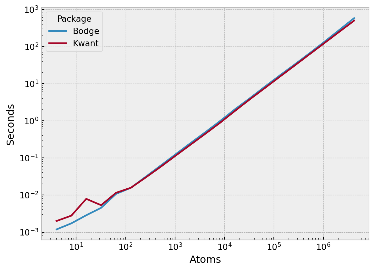
Below, I show some results generated using misc/benchmark.py. This benchmark essentially constructs a non-trivial sparse Hamiltonian matrix for a superconducting system with \(N\) atomic sites using both Bodge and Kwant. The latter is basically the state of the art when it comes to numerical calculations in condensed matter physics and therefore a reasonable benchmark. As you can see, both libraries construct the Hamiltonian in \(\mathcal{O}(N)\) time, in contrast to the \(\mathcal{O}(N^2)\) time one might have expected if one used dense matrices.

import pandas as pd
import seaborn as sns
import matplotlib.pyplot as plt
plt.style.use("bmh")

df = pd.read_csv("misc/benchmark.csv")
sns.lineplot(df, x="Atoms", y="Seconds", hue="Package")
plt.xscale("log")
plt.yscale("log")

On my machine, both libraries can construct a 2D Hamiltonian with one million lattice sites in roughly two minutes. For comparison: To construct this Hamiltonian using dense matrices (NumPy arrays), we would have needed to store \(4N \times 4N\) complex doubles, which would require minimum 256 TB of RAM… Whereas only \((N+4N)(4\times4)\) complex doubles are required for the sparse representation, requiring a bit more than 1 GB of RAM.

Note that Bodge assumes that we are only interested in on-site and nearest-neighbor interactions. This is the most common use case, and constrains the sparsity structure of the resulting Hamiltonian.

Footnotes

1. Examples: Vim has built-in “digraphs” where you can press <C-k>s* in insert mode to type σ. Emacs has a built-in “TeX input method”, which means that after pressing C-\ you can type \sigma to insert the symbol σ. Most other editors code have third-party plugins for this, e.g. Unicode Latex for VSCode. Another option is to use an OS-wide snippet expander (e.g. TextExpander), which you can setup to e.g. convert ;s to a in any application. Another alternative is to just enable a Greek keyboard layout in your OS settings, with a hotkey to switch between the layouts. There are many alternatives!